Loosely speaking, Gaussian processes (GPs) can be thought of as a probabilistic yet non-parametric form of non-linear regression which sit within the Bayesian framework. They are a powerful but less well understood tool that can be used in both a regression and classification setting.

In this article we give a thorough introduction to Gaussian process regression collating many of the excellent references on the topic. We also provide Python code examples.

Introduction

TLDR: GPs give a way to express a view on functions. In particular they allow us to specify how smooth we expect a function to be rather than how many parameters we expect it to have. The key idea they rely on is that data-points that are close in input space are expected to be similar in output space, i.e. if $\mathbf{x}_{i}$ and $\mathbf{x}_{j}$ are similar then $f(\mathbf{x}_{i})$ and $f(\mathbf{x}_{j})$ will be close in value too.

Gaussian processes are Bayesian alternatives to kernel methods and allow us to infer a distribution over functions, which sounds a little crazy but is actually both an intuitive thing to desire as well as being analytically tractable in certain cases.

A typical set-up in supervised machine learning is to start with features $X$ and labels $\mathbf{y}$ and try to find some function $f$ that is a mapping between $X$ and $y$ i.e. $f : X \rightarrow y$. When choosing a model, or functional form for $f$, we are typically fixing the capacity of the model we wish to use. For example, in linear regression, we are assuming there are a fixed number of coefficients and so the total amount of parameters is fixed given the data. Note that this still applies to more powerful models such as neural networks.

What if, instead, we wished to think about all possible functional forms for $f$ without pre-specifying how many parameters are involved? It turns out this is what Gaussian processes allow us to do. In return we must find a way to specify a prior over the type of functions we wish to see.

Outline

We start with a few preliminaries which cover some key prerequisite concepts such as kernel functions, thinking of functions as vectors and a different way to visualize multivariate Gaussians before defining a Gaussian process.

We then walk through the predictive equations for GP regression for the noise-free and noisy case. Next we move onto showing the code and plots for the noisy case which is a simple extension.

Towards the end we detail some helpful mathematical results before a small Q and A section in the appendix which lists some common questions that arose for me whilst developing my understanding of Gaussian processes.

Gaussian process preliminaries

Before defining Gaussian processes it is worth briefly explaining a few concepts, which we do here.

It is also important to be familiar with some of the key properties of multivariate Gaussians and introductory concepts from probability theory such as conditioning and marginalization of variables. These key results are given in the mathematical results section.

Health warning: if you find preliminaries boring feel free to skip to the definition of a Gaussian process below or straight to an example.

Kernel functions

In the context of Gaussian processes a kernel function is a function that takes in two vectors (observations in $\mathbb{R}^ d$) and outputs a similarity scalar between them. For GPs we evaluate the kernel function for each pairwise combination of data-points to retrieve the so-called covariance matrix. As covariance matrices must be positive semi-definite this means valid kernels are those that satisfy this requirement. This covariance matrix, as determined by the kernel function, is essentially what will specify the Gaussian process.

There are many kernels that can describe different classes of functions, including to encode properties such as periodicity. In this post we will restrict ourselves to the most common kernel, the radial basis function (or Gaussian) kernel:

with hyperparameters $\sigma$ and $l$. The variance $\sigma^2$ determines the magnitude of fluctuation of values away from the mean and the length $l^2$ determines the reach of neighbouring data-points (small $l$ will give wiggly functions, increasing $l$ gives smoother functions). See the plot below for the effect of different values of the hyperparameters.

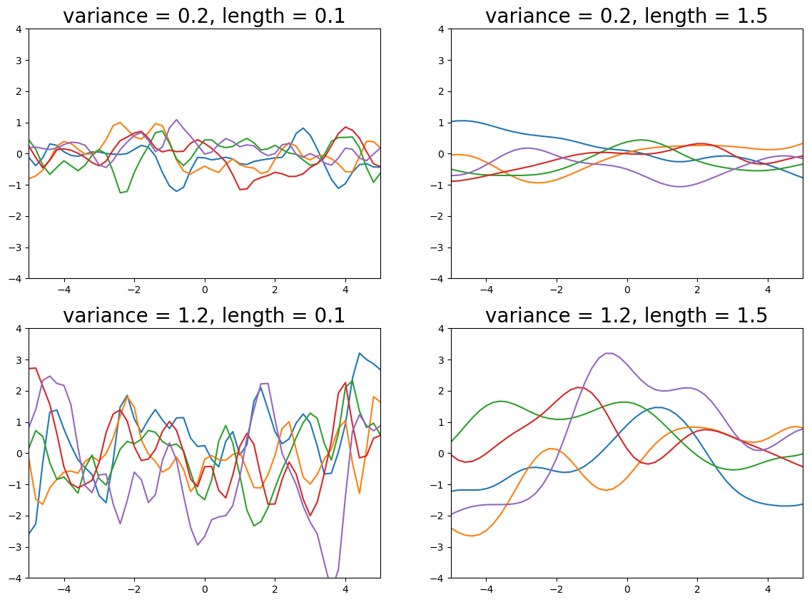
Figure 1. Effect of different kernel hyperparameters

Kernel functions are also sometimes referred to as covariance functions.

Caution: Gaussian processes get their name because they define a Gaussian distribution over a vector of function values, not because they sometimes use a Gaussian kernel to determine the covariances.

Functions as vectors

Loosely speaking a function can be viewed as an infinitely long vector. To do so, we could imagine discretizing the input space with a huge grid of values containing every possible combination of floating point numbers for each of the $d$ dimensions of the data matrix $X$. Theoretically (but not practically) we could then evaluate $\mathbf{f} = (f(\mathbf{x}_{1}), …, f(\mathbf{x}_{n}))$ at this huge sample of $n$ points and thus $\mathbf{f}$ would be an enormous vector containing the function’s values for the domain of interest. For example, if $d=2$ then we can define a grid of points within the bounds of interest for both dimensions and calculate the function value at each point. Note that whilst we will then obtain a vector $\mathbf{f}$ it doesn’t really make sense to think of any ordering within this vector.

Further, we can’t store such a vector containing the function values for every possible input combination (recall each $\mathbf{x_i}$ is $d$ dimensional), though GPs do allow us to define a multivariate Gaussian prior on it. Given partial observations of the elements of this vector, it will turn out that we can infer other elements of the vector without explicitly having to represent the whole object. $\mathbf{f}$.

The miraculous thing about GPs is that they provide a rigorous, elegant and tractable way to deal with the above problem.

Note that whilst talk of functions as vectors may seem a little hand-wavy it can be made rigorous.

A different way to view multivariate distributions

In order to aid the discussion on large dimensional Gaussians it’s crucial to switch to a different way to visualize them. As above we start by thinking of each data-point $\mathbf{x_i}$ as having $d$-dimensions, so $X$ is $n \times d$ dimensional and $\mathbf{x_1}$ and $\mathbf{x_2}$ refer to 2 observations from the data where $\mathbf{y} = \{y_1, y_2\}$ contains the function value for each data-point.

Using the kernel function we can calculate the covariance matrix, $\Sigma$, between these 2 points (using $X$ only, not $\mathbf{y}$), for example:

and by the assumption we make for GPs (see below) we assume the output function values are jointly distributed according to a Gaussian, such that:

Using this idea it is then possible to visualize what the 2-dimensional Gaussian looks like and draw samples from it. Notice that the covariance between the function values is fully specified by the corresponding input values, and not in any way by the function values; this is a property of Gaussian processes.

The left hand plots in the below image show contour/density plots for a 2-dimensional Gaussian with a given correlation coefficient (in reality this will be calculated by the kernel function) and zero mean vector.

The red dots shown in the left hand plots are samples from this 2-dimensional Gaussian.

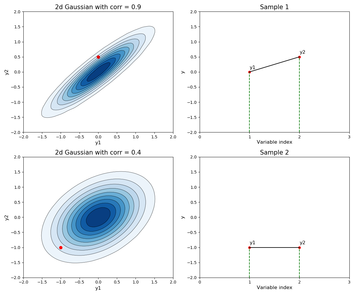
Figure 2. A different way to visualize a sample from a 2-dimensional Gaussian

The right hand plots show an alternate way to visualize this sample, where the y-axis now represent the value of $y_1$ and $y_2$ respectively for each observation $\mathbf{x_1}$ and $\mathbf{x_2}$. In this way we could easily imagine calculating the covariance matrix between more data-points and plotting a sample in the way shown in the right hand plots, but the left hand plots don’t allow this view.

Following this method we could calculate the covariance matrix between 5 observations (a 5-dimensional Gaussian) and sample from it. This way of visualizing the function values is how we are able to represent multi-dimensional Gaussians on a single plot as below:

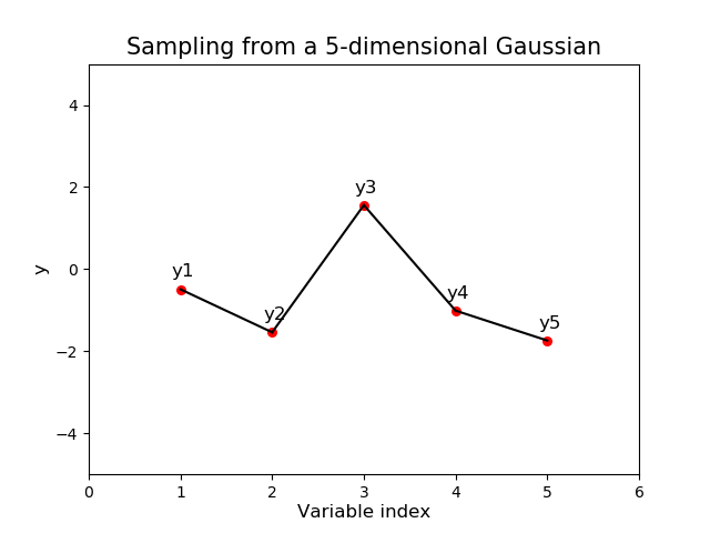
Figure 3. A single sample from a multi-dimensional Gaussian

Hold on, what’s the x-axis for the above plot?

In the above plot we calculated the $5 \times 5$ covariance matrix between 5 points and imagined ordering the points according to their index in the covariance matrix in the above plot. This is simply for illustrative purposes to demonstrate the visualization technique.

In general, the x-axis will be the values of $X$ for which we wish to calculate a point at and thus can take on any real-value. For data with 1 input dimension ($d=1$ and is time, say) this might result in even spacing on the x-axis but this needn’t be the case.

However once $d > 1$ even this view of things breaks down as the input space is now a high-dimensional grid (arbitrarily fine if we wish) for which we can calculate function values at.

Nevertheless, when $d=1$ this way of visualizing helps us plot multi-dimensional Gaussians a lot easier and will be helpful for the examples we encounter in the rest of this post.

Remember: for GPs the multi-dimensional aspect of Gaussians refers to the number of data-points, not the dimensionality, $d$, of $X$.

Posterior predictive

Before we start with the equations for GPs we draw a link to the Bayesian approach which involves inferring the posterior distribution of the parameters of some model given data, i.e. $p(\theta \mid \mathcal{D})$. GPs allow us instead to model $p(f \mid \mathcal{D})$ and we then use this modelled function to predict on new data, $X_{+}$:

and so for each new test point in $X_{+}$ we obtain a probability distribution for the corresponding prediction $\mathbf{y_{+}} $. It turns out for the regression case that the above can be done in closed form using known statistical and linear algebra results.

Whilst the above formulation is useful in linking Gaussian processes into the wider Bayesian framework (by showing a likelihood and a prior) it’s not typically the most intuitive place to start when explaining GPs. For that, it’s much more natural to start by actually defining a Gaussian process and then to rely upon some key properties of the multivariate Gaussian distribution. These are given below and assumed from now on though we will make reference to them as they’re used.

Definition of a Gaussian process

Definition
A Gaussian process is a collection of random variables, any finite number of which have a joint Gaussian distribution.

Note: a Gaussian process is completely specified by its mean function and covariance function.

Thinking of a GP as a Gaussian distribution with an infinitely long mean vector and an infinite by infinite covariance matrix may seem impractical but luckily we are saved by the marginalization property of Gaussians. That is, the whole thing is tractable as long as we only ever ask finite dimensional questions about functions - these finite points are where we have data or wish to predict. The rest of the unseen data is simply integrated out (note we don’t actually need to perform this integration!).

It is also worth reiterating that in the case of Gaussian processes each data point is a random variable and thus the multivariate Gaussian has the same number of dimensions as the number of data-points: for the training data it is a $n$-dimensional Gaussian. Once we add test data for which to predict the multivariate Gaussian will have $n + n_{+}$ dimensions.

We now move onto the predictive equations for the noise-free regression case.

GP regression (noise-free)

We will walk through an example with a small amount of data but the below approach holds for data of any size in theory.

Problem set-up

We start by assuming we are given 3 training data-points which we call $\mathcal{D} = \{ (\mathbf{x_1}, f_1), (\mathbf{x_2}, f_2), (\mathbf{x_3}, f_3)\}$ and a new test point $\mathbf{x_{+}}$ for which we wish to predict the outcome $f_{+}$. We assume that the training data has no noise and contains samples from the true unknown function, that is, $\mathbf{f} = \mathbf{y}$ or $f_i = y_i$ for all $i$.

By the definition of a GP it is assumed that any set of random variables, which are the output function values for the data-points, are distributed as a multivariate Gaussian. Given this assumption we can write the joint distribution between the observed training data and the predicted output as:

It is normally common to assume the mean function is 0 for Gaussian processes, the reasons for why this is are discussed in the Q and A section below.

Sidebar on the covariance sub-matrices
The above sub-matrix $K$ contains the similarity of each training point to every other training point:

\begin{align*} K = \left[ \begin{array}{cc} {K_{11}} & {K_{12}} & {K_{13}} \\ {K_{21}} & {K_{22}} & {K_{23}} \\ {K_{31}} & {K_{32}} & {K_{33}} \end{array} \right] \end{align*}

where each entry $K_{ij} = \kappa(\mathbf{x_i}, \mathbf{x_j})$ is the evaluation of the kernel function between any two data-points. Similarly $K_{+}$ is a $3 \times 1$ vector which contains the evaluation of the similarity between each training data-point and the test point $\mathbf{x_{+}}$. $K_{\\++}$ in this case is a scalar with the similarity between the test point to itself.

The above generalizes to many data-points and in general $K$ has dimensions $n \times n$, $K_{+}$ has dimensions $n \times n_{+}$ and $K_{\\++}$ has dimensions $n_{+} \times n_{+}$.

Prediction: condition then marginalize

Using the properties of multivariate Gaussians we are able to write down the predictive equations for GPs. Note that in contrast to other Bayesian analysis we do not need to trouble ourselves with computing a posterior explicitly, nor do we need to perform any integration.

Instead we condition on the observed training data, $\mathbf{f}$, to obtain the posterior predictive distribution for $f_{+}$. Using the result for the conditioning of Gaussians we have, for a single test point:

The above conditioning reduces a 4-dimensional Gaussian down to a 1-dimensional Gaussian - we can thus think of the conditioning as cutting 3 slices in the 4-dimensional space to leave us with a 1-dimensional distribution. In general, once we have conditioned on the observed data we will be left with a multivariate Gaussian with dimensionality equal to the number of test points we wish to predict for, $n_{+}$.

To then obtain the marginal distribution of each test point we use the marginalization property of multivariate Gaussians to obtain the mean prediction and variance estimate for each point (in this case there is no need to as, starting with only one test point, we are automatically left with a 1-dimensional distribution).

In this way the prediction is not just an estimate for that point, but also has uncertainty information - for understanding why estimating uncertainty is important see the Q and A below.

Sidebar on interpreting the predictive equations
Equation (4) above for the predictive mean was given as:

\begin{align*} \mathbf{\mu}_{f_{+} \mid \mathbf{f}} &= \color{#e5c07b}{\mu\left(\mathbf{x_{+}}\right)} + \color{#e06c75}{K_{+}^{T}} \color{#98c379}{K^{-1}}\color{#c678dd}{(\mathbf{f} - \mu(X)) } \end{align*}

which can be intepreted as the prior guess we had for the mean of the test point before seeing any data plus the surprise/difference in the observed data from what we expected normalized by the training data's variance which is then weighted by how similar the training and test data are.

Similarly for equation (5) and the predictive variance:

\begin{align*} \Sigma_{f_{+} \mid \mathbf{f}} &= \color{#e5c07b}{K_{\\++}}- \color{#e06c75}{K_{+}^{T}} \color{#98c379}{K^{-1}} \color{#e06c75}{K_{+}} \end{align*}

can be interpreted as the prior guess we had for the variance of the test data before seeing any data minus a reduction in uncertainty based on how similar the training and test data are normalized by the training data's variance.

Adding more data

In the above we have 3 observed data-points and made a prediction for a single new test point. If we wish to predict for more test data we can simply repeat the above steps and thus we are able to get probabilistic predictions for any number of test points. In a similar spirit if we observe new training data we can add this in to $X$ and recalculate the predictions for the test points. (Note this ignores computational considerations to keep things simple.)

Walking through an example with plots

We now give an example to illustrate the above discussion.

In this example we are given 3 training data-points as $(x, y)$ pairs with $\mathcal{D} = \{(-2, 1), (1, -1.5), (4, 2)\}$ and a new test point $x_{+} = 3$ and we wish to predict $f_{+} = f(3)$.

The below chart visualizes parts of the GP fit process and is explained below:

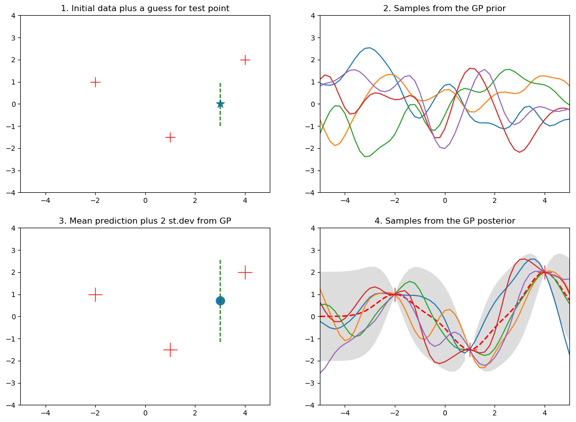
Figure 4. Gaussian process fit plots

Subplot 1: just the data

Without a model and by visually inspecting the 3 training data-points we might guess that $f_{+} \approx 0$ and we might also perhaps expect it to lie in some range around this point. This is an informal way of thinking about the key idea behind GPs - that we expect points that are close in input space to also be close in output space.

Subplot 2: sampling from the prior

By defining the kernel function, and before observing any training data, we are specifying a view on how smooth/wiggly we expect the estimated functions to be. Sampling from the prior amounts to having to specify some domain of interest (here we use -5 to 5) and discretizing it into many points. This is what we loosely mean by saying a function is just a vector of values. This subplot essentially shows a 50-dimensional Gaussian as this is the number of points used along the x-axis - note this creates realistic plots and is a key point. We rarely ever care about every single value the input data can take but just a subset where we have training data or wish to predict.

The data for this subplot is not part of the training data and we just show these samples for illustration. This distribution over functions will become constrained once we observe some data.

Subplot 3: fit the Gaussian process

Here we have fit the GP regression model and show the outcome. The blue dot is the mean value for the GP prediction and the green dashed line shows $\pm 2$ standard deviations around the predicted mean value.

Subplot 4: sampling from the posterior

Similar to what we did when we sampled from the prior we can predict the GP for a range of $x$ values, here we do it for many points along the x-axis and show the resulting mean vector (red-dashed line) and $\pm 2$ standard deviation estimates for the mean prediction at each $x$ point. Note that where we have observed data the functions from the posterior are constrained to go through the data but in the places where we have no data the possible function fits are many and varied.

Comment

Recall that we can represent a function as a big vector where we assume this unknown vector was drawn from a big correlated Gaussian distribution, this is a Gaussian process. As we observe elements of the vector this constraints the values the function can take and by conditioning we are able to create a posterior distribution for functions. This posterior is also Gaussian and so the posterior over functions is still a Gaussian process. The marginalisation property of Gaussian distributions allows us to only work with the finite set of function instantiations $\mathbf{f} = (f(\mathbf{x}_{1}), …, f(\mathbf{x}_{n}))$ which constitute the observed data and jointly follow a marginal Gaussian distribution.

GP regression (noisy)

Having walked through the noise-free case the extension to the noisy case is straightforward. We now assume that the observed data is a noisy version of the true underlying function and instead we now observe training data $\mathcal{D}$ where, for a single point $i$, we have

and $\epsilon$ is additive independent identically distributed Gaussian noise such that $\epsilon \sim \mathcal{N}(0, \sigma_y^2)$.

The goal is still to predict $f_{+}$ for a single test point or $\mathbf{f_{+}}$ for many test points.

Given this noise assumption the only difference in the joint distribution with the noise-free case is on the prior of the noisy observations.

where here we are assuming a 0 mean vector.

Sidebar: covariance terms
Under the independent identically distributed Gaussian noise assumption only a diagonal matrix is added to the noisy observed terms. We can see this by recalling a property of covariance:

\begin{align*} \operatorname{cov}(X+Y, W+V)=\operatorname{cov}(X, W)+\operatorname{cov}(X, V)+\operatorname{cov}(Y, W)+ \operatorname{cov}(Y, V) \end{align*}

and for $\operatorname{cov}(\mathbf{y}, \mathbf{y})$ we have for a single point $i$:

\begin{align*} \operatorname{cov}(f(\mathbf{x_i}) + \epsilon, f(\mathbf{x_i}) + \epsilon) = \underbrace{\operatorname{cov}(f(\mathbf{x_i}), f(\mathbf{x_i}))}_\text{$K(X, X)$} + \underbrace{\operatorname{cov}(f(\mathbf{x_i}), \epsilon)}_\text{= 0} + \underbrace{\operatorname{cov}(\epsilon, f(\mathbf{x_i}))}_\text{= 0} + \underbrace{\operatorname{cov}(\epsilon, \epsilon)}_\text{$\sigma_y^2$} \end{align*}

Similar reasoning means the noise term will not contribute to the $\operatorname{cov}(\mathbf{y}, \mathbf{f_{+}})$, $\operatorname{cov}(\mathbf{f_{+}}, \mathbf{y})$ or $\operatorname{cov}(\mathbf{f_{+}}, \mathbf{f_{+}})$ terms.

Predictive equations: noisy case

A similar conditioning argument leads to the predictive equations in the noisy case with 0 mean for a vector of predictions, $\mathbf{f_{+}}$:

As in the noise free case we use the marginalization property of multivariate Gaussians to obtain a mean prediction and variance estimate for each test point in the vector $\mathbf{f_{+}}$.

Next we move onto something more practical, actually fitting a GP for a noisy regression case!

Algorithm for GP regression

We now walk through an example with Python code detailing how to actually fit a Gaussian process for regression with noise. We start by defining the algorithm before supplying code and charts.

---

Algorithm: GP regression

---

1. $L = \operatorname{cholesky}(K + \sigma_{y}^2 \, I)$
2. $\alpha=L^{T} \backslash(L \backslash \mathbf{y})$
3. $\mathbb{E}\left[\mathbf{f_{+}}\right]=K_{+}^{T} \alpha$
4. $v = L \backslash K_{+}$
5. $\operatorname{var}\left[\mathbf{f_{+}}\right]=K_{ \\++}-v^{T} v$

Note the solution to $A\mathbf{x} = \mathbf{b}$ is often denoted as $A \backslash \mathbf{b}$.

The Cholesky decomposition provides a more numerically stable alternate to directly inverting $K$. For more on the use of the Cholesky decomposition see the Q and A section below.

Problem set-up

Given 10 noisy observations from a sine wave over the domain $(-5, 5)$, predict the function for an evenly spaced set of 50 points over the same domain. The red crosses are the training data-points and the blue curve shows the true unknown function for illustrative purposes. In plot 3 the red dashed line is the mean prediction for the 50 test points.

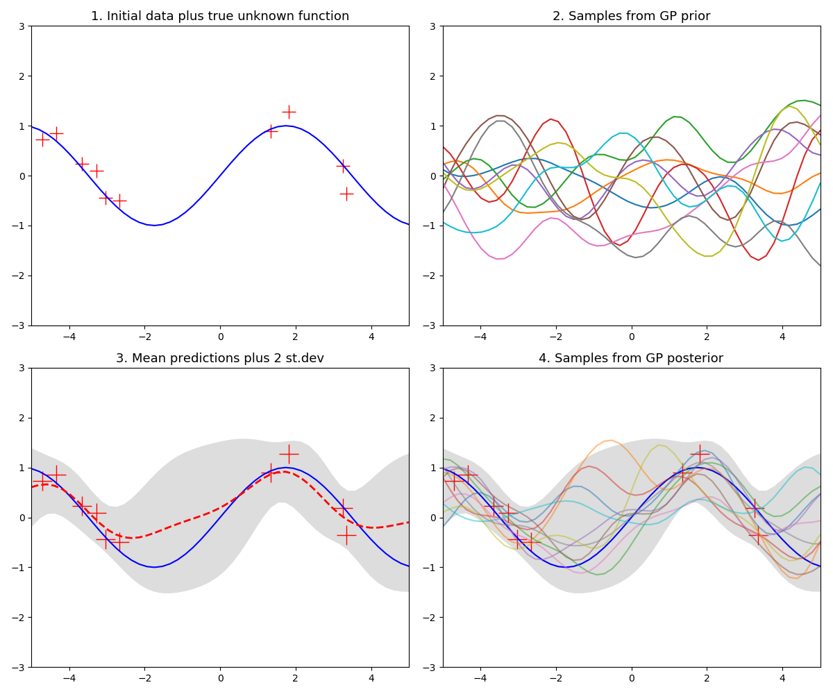
Figure 5. Gaussian process example with limited data for a sine wave

Comments on the above GP fit

Python code

Example python code of the GP example (excludes plotting code):

import numpy as np

def kernel(a, b, variance=0.5, length=1):
    """GP squared exponential kernel for 1d inputs: the similarity function"""
    sqdist = np.sum(a**2,1).reshape(-1,1) + np.sum(b**2,1) - 2*np.dot(a, b.T)
    return np.exp(-.5 * (1/length) * sqdist) * variance

f = lambda x: np.sin(0.9*x).flatten()  # true unknown function to approx

n_train, n_test = 10, 50     # number training & test points
n_prior_samples, n_post_samples = 10, 10
s = 0.2    # noise variance to create data with

# 1. Compute prior over test domain
X_test = np.linspace(-5, 5, n_test).reshape(-1,1)
K_ss = kernel(X_test, X_test)
L_prior = np.linalg.cholesky(K_ss + 1e-6*np.eye(n_test))
f_prior = np.dot(L_prior, np.random.normal(size=(n_test, n_prior_samples)))

# 2. Create noisy training data and compute kernel function for training data
X = np.random.uniform(-5, 5, size=(n_train, 1))
y = f(X) + s*np.random.randn(n_train)
K = kernel(X, X)
L = np.linalg.cholesky(K + s*np.eye(n_train))  # K = LL^T

# 3. Compute kernel function between train and test data
alpha = np.linalg.solve(np.dot(L, L.T), y)
K_s = kernel(X, X_test)

# 4. Get mean prediction and uncertainty for each test point
mu = np.dot(K_s.T, alpha)
L_k = np.linalg.solve(L, K_s)
s_var = np.diag(K_ss) - np.sum(L_k**2, axis=0)
stdev = np.sqrt(s_var)

# 5. Optional: sample from the posterior at test points
L_post = np.linalg.cholesky(K_ss + 1e-6*np.eye(n_test) - np.dot(L_k.T, L_k))
f_post = mu.reshape(-1,1) + np.dot(L_post, np.random.normal(size=(n_test, n_post_samples)))

Helpful mathematical results

Multivariate Gaussians - key results

We do not give an exhaustive overview of the many properties of multivariate Gaussians but instead give a few key properties which are of paramount importance for the use of Gaussian processes.

Marginalization property: marginal of a joint Gaussian is Gaussian
Let $X = (x_1, ..., x_n)$ and $Y = (y_1, ..., y_n)$ be jointly distributed Gaussian random variables:

\begin{align*} p(X, Y) = \mathcal{N} \Bigg( \left[ \begin{array}{c}{\boldsymbol{\mu}_X} \\ {\boldsymbol{\mu}_Y}\end{array}\right] \, , \, \left[ \begin{array}{cc}{\Sigma_{XX}} & {\Sigma_{XY}} \\ {\Sigma_{YX}} & {\Sigma_{YY}} \end{array}\right] \Bigg) \end{align*}

then the marginal distribution is Gaussian

\begin{align*} p(X) &= \int p(X, Y) \, dY \\[5pt] &= \mathcal{N}(\boldsymbol{\mu}_X , \Sigma_{XX}) \end{align*}

Conditioning property: conditional of a joint Gaussian is Gaussian
It is also the case that:

\begin{align*} X \mid Y \sim \mathcal{N}\left(\boldsymbol{\mu}_{X}+\Sigma_{X Y} \Sigma_{YY}^{-1}\left(Y - \boldsymbol{\mu}_{Y}\right), \Sigma_{X X}-\Sigma_{X Y} \Sigma_{YY}^{-1} \Sigma_{Y X}\right) \end{align*}

and so conditioning also gives us a Gaussian.

For references on how to derive the first two results see CS229 notes here.

Product of two Gaussian densities is an (unnormalized) Gaussian

\begin{align*} \mathcal{N}(\mathbf{x} ; \mathbf{a}, A) \mathcal{N}(\mathbf{x} ; \mathbf{b}, B)=Z^{-1} \mathcal{N}(\mathbf{x} ; \mathbf{c}, C) \end{align*}

where

\begin{align*} \mathbf{c}=C\left(A^{-1} \mathbf{a}+B^{-1} \mathbf{b}\right) \quad \text { and } \quad C=\left(A^{-1}+B^{-1}\right)^{-1} \end{align*}

with the normalizing constant itself looking Gaussian:

\begin{align*} Z^{-1}=(2 \pi)^{-D / 2}|A+B|^{-1 / 2} \exp \left(-\frac{1}{2}(\mathbf{a}-\mathbf{b})^{\top}(A+B)^{-1}(\mathbf{a}-\mathbf{b})\right) \end{align*}

See Rasmussen [A.7] for more details.

Note that the product of two Gaussian random variables (not densities) is not necessarily Gaussian.

References

In order to get a grip on the basics of GPs I read many sources, most listed below.

Books and papers

Videos and/or presentation slides

Blogs and web articles

Appendix Q and A

This section contains some questions and answers that may arise whilst learning about GPs for the first time.

What is a collection of random variables?

Collections of random variables are stochastic processes, the most common of which is the random walk. A Gaussian process is a stochastic process such that every finite collection of those random variables has a multivariate normal distribution.

Why is the mean function often set to 0 in the prior?

Even if we set the mean function to 0 in the prior the predicted mean for a test data-point will not be 0. To see this recall the predictive mean becomes:

even if we set the prior mean function $\mu_i = 0$ for all $i$. Thus the predictive mean depends on the kernel and on the number of training points and so can be arbitrarily flexible. It is worth noting that for predictions far away from the training data and dependent upon the kernel (and its hyperparameters) a GP may still predict $f_{+} \approx 0$ if a point $x_{+}$ is sufficiently far from the training set. However this is not a bad idea in general and can stop wild predictions when extrapolating far from the observed data.

Practically when fitting GPs it is desirable to standardize the data (function values, not $X$) to have 0 mean. It can also be advisable to normalize $X$ too depending on the kernel function.

How can we set the kernel hyperparameters?

The kernel hyperparameters control the type of functions GPs can produce and yet we have not talked at all so far about how to set them! We amend that now and will mention one common way but many more exist (e.g. cross-validation). Recall that the kernel function dictates the prior beliefs we have about the type of functions we expect to fit the data well.

Empirical Bayes

The empirical Bayes approach is a popular method for choosing how to set the prior that involves estimating it from the data. In this way some Bayesians philosophically disagree with the use of empirical Bayes methods as the prior will no longer represent the view we have about functions before seeing the data. As well as the kernel hyperparameters there is also a choice to be made as to which is the appropriate choice of kernel, though we do not discuss this topic in this post.

In order to perform empirical Bayes for GP regression we maximize the marginal likelihood, or equivalently marginal log-likelihood, of the data which is given by:

The term marginal likelihood is used to refer to the marginalization over the function values $\mathbf{f}$. For a GP the prior is a Gaussian

and so

The likelihood is also Gaussian:

Given the above it is possible to perform the integration of $(11)$ by using the fact that the product of two Gaussian densities gives another (unnormalized) Gaussian. This allows us to obtain

an expression for the log marginal likelihood. Depending on the kernel function we chose we are now able to now compute its derivative with respect to each hyperparameter and then to estimate the hyperparameters using any standard gradient-based optimizer. However, since the objective is not convex, local minima can be a problem.

For more reading on this topic please see Rasmussen chapter 5.

Why is knowing the uncertainty important?

Often in the real-world we (should) care not just about the mean prediction but also the amount by which it could vary. Further, knowing where we are most uncertain can be helpful if we have to make a decision about where to next obtain a sample which is expensive to compute. Examples of expensive functions could be drilling a well, conducting a clinical trial or training a large neural network.

Using uncertainty in a probabilistic model to guide search is called Bayesian optimization and commonly uses Gaussian processes.

How can we sample from a multivariate Gaussian

Sampling from an arbitrary distribution usually involves computing the CDF of the distribution, which may not be feasible and for a Gaussian there is famously no closed form solution. However most software packages will have an implementation of an efficient way to sample from a standard Gaussian, $\mathcal{N}(0, 1)$.

Broadly speaking it will be much more efficient if we can relate everything to a standard Gaussian. In 1-dimension we can use the fact that $x \sim \mathcal{N}(\mu, \sigma^2)$ can be written as $x \sim \mu + \sigma \mathcal{N}(0, 1)$ and use this fact to sample from a Gaussian with arbitrary mean and variance by sampling from $\mathcal{N}(0, 1)$ instead.

To generalize this idea to sample from multi-dimensional correlated random variables $X \sim \mathcal{N}(\boldsymbol{\mu}, \Sigma)$ we would like to be able to sample from $X \sim \boldsymbol{\mu} + L \, \mathcal{N}(0, I)$ for some $L$. This $L$ needs to be computable and the equivalent to the square-root of the covariance matrix, i.e. a matrix $L$ such that $LL^T = \Sigma$.

$L$ is exactly what the Cholesky decomposition gives us.

In this way we can sample from $X \sim \mathcal{N}(\boldsymbol{\mu}, \Sigma)$ using $X \sim \boldsymbol{\mu} + L \, \mathcal{N}(0, I)$.

This is a standard result but discussion is provided in Rasmussen [A.2].

Inverse sampling transform

The idea behind the above relates to the inverse sampling transform algorithm.

---

Algorithm: Inverse sampling transform

---

Inverse transform sampling is a method for sampling from any distribution given its CDF, $F_X(x)$.

1. Generate a random number $u$ from the uniform distribution on $[0, 1]$.
2. Compute the inverse of the CDF as, $F_X^{-1}(u)$.
3. $F_X^{-1}(u)$ is from the target distribution.

Why do we assume correlation between observations?

When forming a prior over functions we somehow must define a way to construct a covariance matrix. Clearly we don’t want to specify anything manually and we’d like to use the belief that points in input space that are similar have function values that are similar, in other words, the function has some form of smoothness. This is a reasonable assumption for most real world phenomena.

If we used a diagonal covariance matrix then it would be the same as saying we believed the function values to be independent and so observing the function in one location would tell us nothing about its values in other locations. Given we usually want to model continuous functions we would like function values for more similar inputs to be closely related.

Why are GPs non-parametric?

To quote wikipedia:

Non-parametric models differ from parametric models in that the model structure is not specified a priori but is instead determined from data. The term non-parametric is not meant to imply that such models completely lack parameters but that the number and nature of the parameters are flexible and not fixed in advance.

GPs are non-parametric models and technically have an infinite number of parameters (given by the infinite mean vector and covariance matrix) which are integrated out by the marginalization property of Gaussians.

As we add more data the flexibility and capacity of the model will adjust to fit the data: we would see the mean function adjust itself to pass close to these points, and the posterior uncertainty would reduce close to the observations.

In this way we do not have to worry about whether it is possible for the model to fit the data - the complexity of the model adjusts naturally with the data.